zkMIPS Overview

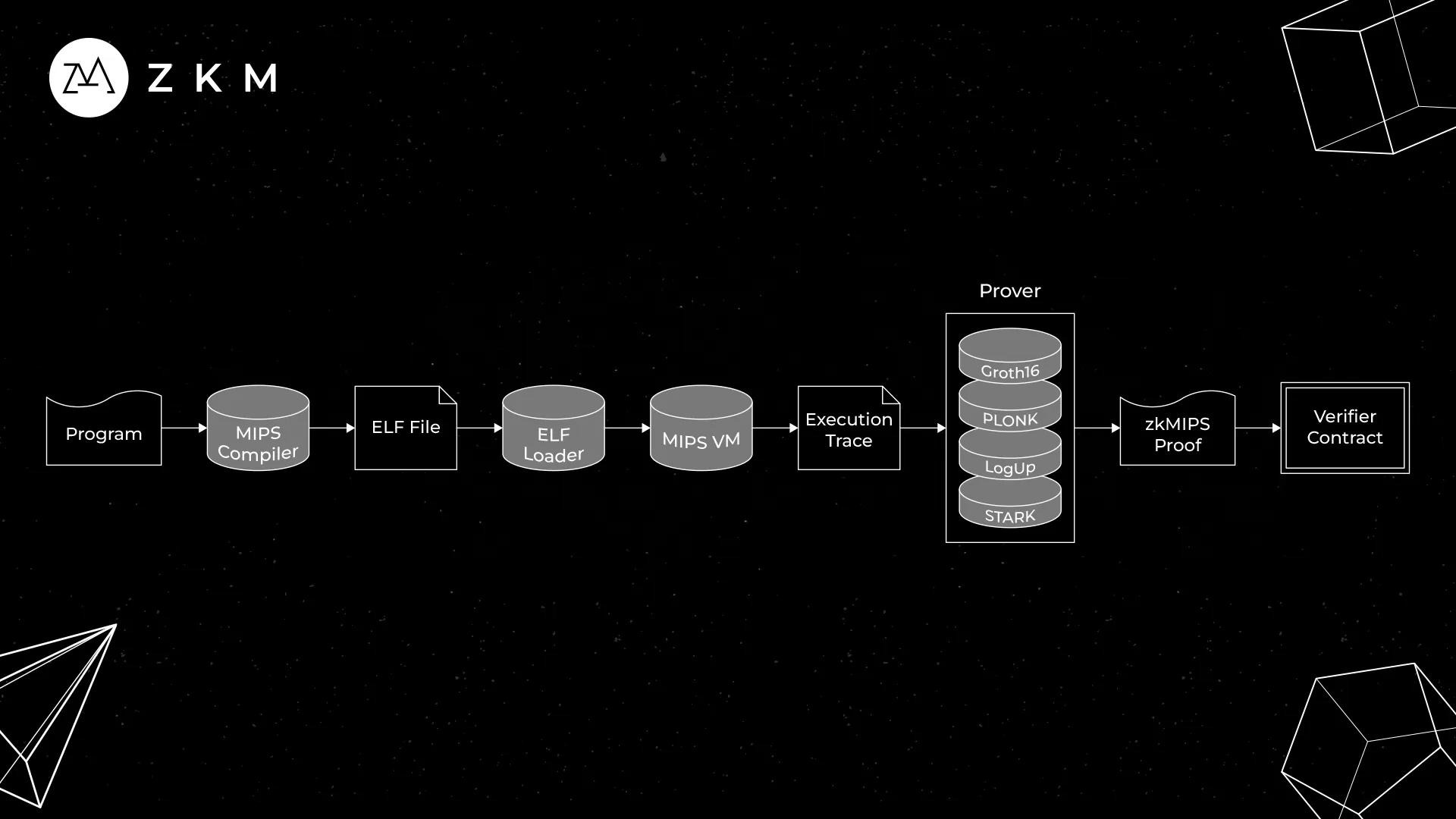
Overview of the zkMIPS architecture for proving the execution of a program

Proofs of Knowledge (opens in a new tab) in verifiable computation involve a Prover that performs a computation and produces a proof to show this computation was correctly executed, both of which are sent to the Verifier.

The proof should be short or “succinct” so that the Verifier has minimal work to do. This is however at the cost of putting the burden on the Prover.

Proofs of knowledge within blockchains are:

1. Succinct

2. Non-interactive (between the Prover and Verifier)

3. ZK (this is optional). Common computational problems that are usually proven are ^{[3] (opens in a new tab)}:

   1. Transition functions for L2s – as seen in zkRollups.
   2. The execution of smart contracts – as seen in zkEVMs. Smart contracts are typically written in Solidity and the EVM verifies the execution of the contract.
   3. The execution of off-chain programs – as seen in zkVMs. In ZKM’s case, an off-chain MIPS program is given and zkMIPS verifies the execution of that program on-chain.

zkMIPS in Verifiable Computation

zkMIPS verifies the correctness of the execution of a MIPS program in the form of a proof. This is equivalent to the sequence of overall CPU states that represent a program’s execution.

In zkMIPS, the computational problem that we want to verify is the program. The solution comes in the form of an execution trace (opens in a new tab).

An execution trace is a complete record of the computation executed from running the program. The execution trace is commonly represented through a trace record, where each column is a list representing the states of a fixed CPU variable and the rows showing each step of the computation.^{[1] (opens in a new tab)}

The program is verified by checking whether each row of the execution trace matches the respective instruction of a program.

A solution to this is to simply rerun the program. The problem is that this is not succinct. Similar to what we’ve discussed with the trivial proofs (opens in a new tab) in proofs of knowledge, the state sequences would be too large for the smart contract to verify.^{[2] (opens in a new tab)}

Techniques For Succinct zkMIPS Proving

The following sections describe techniques that zkMIPS uses for improving the succinctness during the proof generation process. This includes arithmetization, FRI, method continuation, lookups and polynomial commitments.

More details can be found in “Getting to Know zkMIPS Proving Architecture” (opens in a new tab) written by ZKM Researcher Lucas Fraga and the zkMIPS whitepaper (opens in a new tab) written by the ZKM research team.

How can we complete the verification of a MIPS program more efficiently?

With succinct proofs (opens in a new tab), we can verify a program in a time that is polynomial on the logarithm of the size of the program. For example, a program of size n can be verified in around a time that is polynomial on log(n).

To enable greater succinctness, zkMIPS uses 2 main methods:

1. Compressing the number of verification steps
2. Moving the verification complexity from the Verifier to the Prover (hence there is a sophisticated Prover and a simple Verifier).

Arithmetization

In moving the verification complexity to the Prover, we can use polynomials. Using arithmetization, we can represent the entire trace record as a single polynomial.

The constraints (verification steps) and witnesses (the values in each step) can be encoded as polynomials. The constraint and witness polynomials can be combined together to form a single composition polynomial.

In the above diagram, the MIPS instructions and registers are encoded as polynomials. Constraints are applied in each row of the trace table. Each row is then converted into a constraint polynomial.

We can now:

1. Combine the different steps of the program and compress them
2. Combine the constraint and witness polynomials into a single function where the result should still be a polynomial if the constraint and witness polynomials match.

The program is verified through polynomial evaluations on the composition polynomial. What specific evaluations should be performed on the composition polynomial?

FRI Protocol

The FRI protocol is one such method for determining this, specifically used to verify whether the composition polynomial has a proper degree.

The way the composition polynomial is defined guarantees that, if it is indeed a polynomial, the witness and constraints must match, and the program and its execution trace as a result are compatible. This is sufficient enough to verify the program.

There are, however, problems to creating a composition polynomial for the entire program:

1. The polynomial input to FRI can be as large as the MIPS program
2. FRI proofs are heavily based on hash functions, which are expensive to compute on-chain

Using FRI alone is not succinct enough for on-chain verification.

Lookup Protocols

A lookup protocol shows that a target table is contained in a reference table, i.e., that the segment is contained in the modular tables.

The lookup protocol, if successful, shows that every entry in the original set of internal CPU states appears in the table of one of the operation groups. The lookup proof will be equivalent to the FRI-based continuation proof.

Lookups are used because:

1. They are another technique to improve succinct proving by decreasing the proof size
2. Some operations (e.g., logic operations) cannot easily be expressed as polynomials

Different tables are created for different types of operations and table lookups are used to show the original segment table corresponds to the smaller operation tables proved with FRI. Different programs will also produce different tables. The entries of the tables and lookups into the tables are encoded as polynomials.

In zkMIPS, the segment polynomials are broken down into four main modular tables: arithmetic, logic, memory and control. FRI is used to prove each operation group in parallel and joins them together in a lookup protocol.

There are two types of tables used:

• Target table – a table representing the entire segment
• Reference table – a table combining all four modular tables

Continuation

To counter the computational expense of creating a single composition polynomial, method continuation can be used by breaking down the witness and constraint polynomials into pieces.

This process includes:

1. Dividing the program into smaller segments
2. Proving each of the segments in parallel
3. Running the FRI protocol for each segment
4. Combining all segments proofs to get a program proof

We will end up with one FRI proof for each segment. The continuation protocol will show that the FRI proofs continue onto one another, which is done recursively until there is one single continuation proof. The final proof will be around the size of one segment proof and is sufficient enough to prove the correctness of the entire program.

Because the resulting continuation proof is FRI-based, it is not adequate for on-chain computation. We can further improve the succinctness by using lookups.

Polynomial Commitments

Polynomial commitments are used to further decrease the overall final proof size and proving time by adjusting the FRI-produced proofs.

Using polynomial commitments, larger proofs can be produced faster and smaller proofs can be produced slower. The last continuation proof uses slow and small commitments (to decrease the final proof size) before being converted into Groth16. The other FRI-based phases use fast and large commitments.

Another note about polynomial commitments: zkMIPS uses Merkle trees to commit to all possible evaluations of certain polynomials in a given domain. The Verifier can use the Merkle root to query the polynomial evaluation from the Prover and check certain polynomial properties using the queried values.^{[1] (opens in a new tab)}